Usage
continuum_mechanics relies on SymPy
for symbolic calculations. To use Continuum Mechanics in a project you can
import it as:
import continuum_mechanics
Vector operators in Cartesian coordinates
continuum_mechanics support major vector operators such as:
- gradient of a scalar function;
- divergence of a vector function;
- curl of a vector function;
- gradient of a vector function;
- divergence of a tensor;
- Laplace operator of a scalar function;
- Laplace operator of a vector function; and
- Biharmonic operator of a scalar function.
All these operators are in the module vector.
from sympy import *
from continuum_mechanics import vector
By default, Cartesian coordinates are given by \(x\), \(y\) and \(z\). If these coordinates are used there is not necessary to specify them when calling the vector operators
init_printing()
x, y, z = symbols("x y z")
Following, we have some examples of vector operators in Cartesian coordinates.
Gradient of a scalar function
The gradient takes as input a scalar and returns a vector, represented by a 3 by 1 matrix.
f = 2*x + 3*y**2 - sin(z)
f
vector.grad(f)
Divergence of a vector function
The divergence takes as input a vector (represented by a 3 by 1 matrix) and returns a scalar.
vector.div(Matrix([x, y, z]))
vector.div(Matrix([
    x**2 + y*z,
    y**2 + x*z,
    z**2 + x*y]))
Divergence of a tensor function
The divergence of a tensor (represented by a 3 by 3 matrix) returns a vector.
Axx, Axy, Axz = symbols("A_xx A_xy A_xz", cls=Function)
Ayx, Ayy, Ayz = symbols("A_yx A_yy A_yz", cls=Function)
Azx, Azy, Azz = symbols("A_zx A_zy A_zz", cls=Function)
tensor = Matrix([
    [Axx(x, y, z), Axy(x, y, z), Axz(x, y, z)],
    [Ayx(x, y, z), Ayy(x, y, z), Ayz(x, y, z)],
    [Azx(x, y, z), Azy(x, y, z), Azz(x, y, z)]])
tensor
vector.div_tensor(tensor)
Curl of a vector function
Let us check the identity
fun = symbols("fun", cls=Function)
vector.curl(vector.grad(fun(x, y, z)))
Visualization of tensors
from sympy import Matrix
from continuum_mechanics.visualization import mohr2d, mohr3d, traction_circle
Visualization in 2D
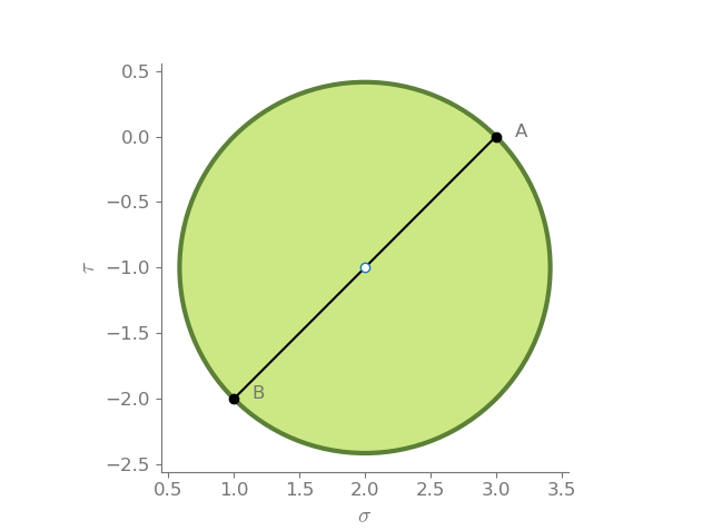
First, let us visualize the tensor
mohr2d(Matrix([
  [1,0],
  [0,-1]]))
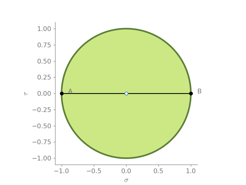
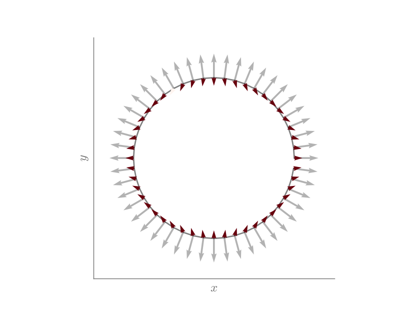
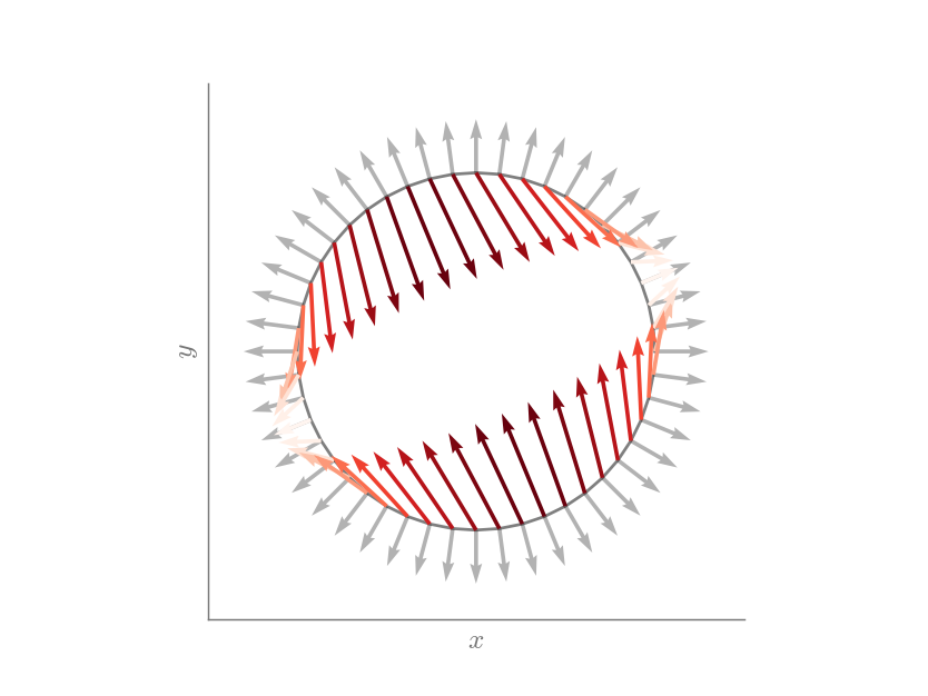
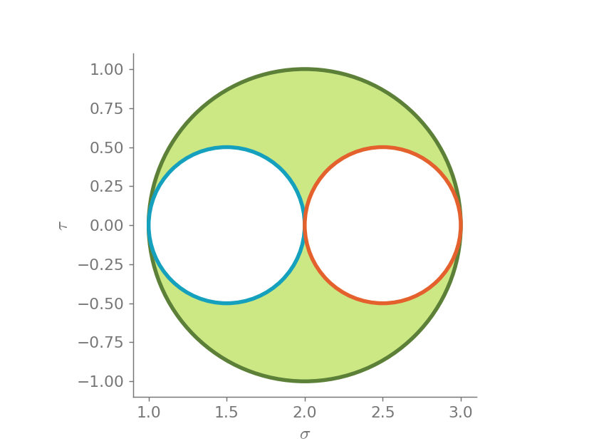
From the Mohr circle, we can see that the principal directions are given at \(0\) and \(\pi/2\) radians. This can be more easily visualized using the traction circle, where normal vectors are presented in light gray and the traction vectors are presented in colors.
traction_circle(Matrix([
  [1,0],
  [0,-1]]))
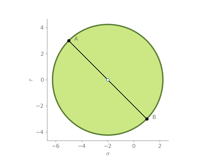
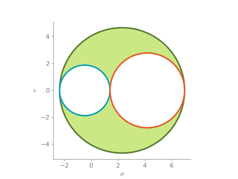
Now, let us visualize
mohr2d(Matrix([
  [1, 3],
  [3, -5]]))
traction_circle(Matrix([
  [1, 3],
  [3, -5]]))
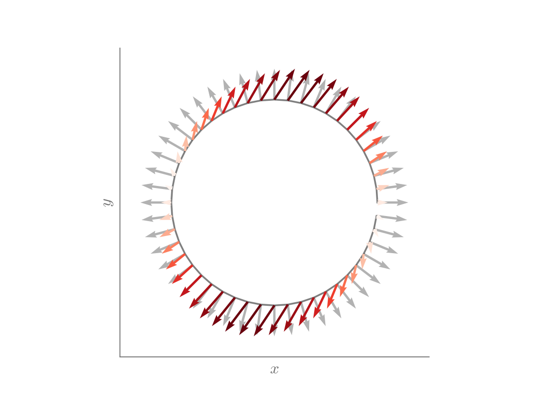
Now, let us try it with an asymmetric tensor
mohr2d(Matrix([
  [1, 2],
  [0, 3]]))
traction_circle(Matrix([
  [1, 2],
  [0, 3]]))
Mohr Circle in 3D
Let us visualize the tensor
mohr3d(Matrix([
    [1, 2, 4],
    [2, 2, 1],
    [4, 1, 3]]))
Now, let us visualize the tensor
mohr3d(Matrix([
    [1, 0, 0],
    [0, 2, 0],
    [0, 0, 3]]))
Elasticity tensor visualization
Let us consider β-brass that is a cubic material and has the following material properties in Voigt notation:
C11 = 52e9
C12 = 27.5e9
C44 = 173e9
rho = 7600
C = np.zeros((6, 6))
C[0:3, 0:3] = np.array([[C11, C12, C12],
                        [C12, C11, C12],
                        [C12, C12, C11]])
C[3:6, 3:6] = np.diag([C44, C44, C44])
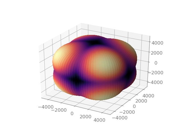
One way to visualize a stiffness tensor is to use the Christofel equation
where \(\Gamma_{ij}\) is the Christofel stiffness and depends on the material properties (\(c_{ijkl}\)) and unit vectors (:math`n_i`):
This provides the eigenvalues that represent the phase speed for three propagation modes in the material.
V1, V2, V3, phi_vec, theta_vec = christofel_eig(C, 100, 100)
V1 = np.sqrt(V1/rho)
V2 = np.sqrt(V2/rho)
V3 = np.sqrt(V3/rho)
Phase speed for the first quasi-transverse mode.
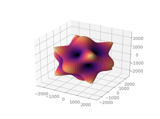
Phase speed for the second quasi-transverse mode.
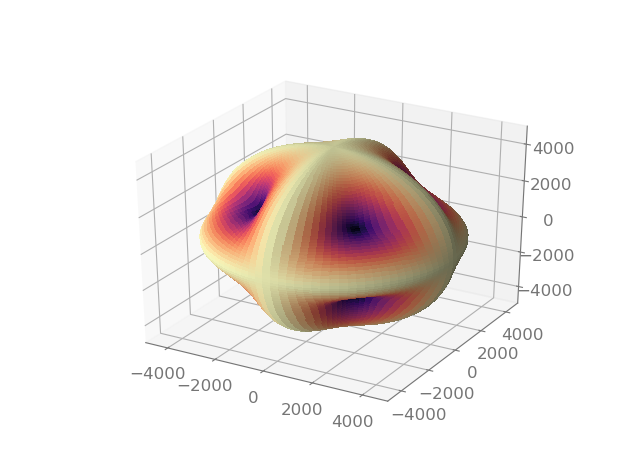
Phase speed for the quasi-longitudinal mode.